FEM with Ferrite in Julia

Making a Mesh with GMesh

You can download GMesh and it’s GUI here. You can play with this a bit on it’s own to get used to generating meshes.

From inside Julia we use GMesh through FerriteGmsh.jl

Lets make a sphere.

using Ferrite, FerriteGmsh

gmsh.initialize() #Initialize Gmsh
mesh_size = 0.1 # A smaller value will result in a finer mesh

#Define the sphere (x, y, z, radius)
sphere_tag = gmsh.model.occ.addSphere(0.0, 0.0, 0.0, 1.0)
gmsh.model.occ.synchronize()
gmsh.model.mesh.generate(3) #why does this have a 3?

grid = togrid() #Convert the Gmsh model to a Ferrite Grid
gmsh.finalize() #Finalize Gmsh to free resources

#Save the grid to a VTK file for Paraview
#The file will be named "sphere.vtu"
vtk_grid("sphere", grid) do vtk
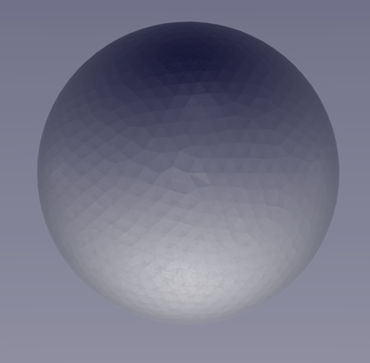
end

To view the sphere, download ParaView . Drag and drop your .msh file into Paraview, and voila! A sphere.

This tutorial is for people who want a complete explanation of the method, and have some patience for mathamatics, but don’t have a strong math or physics background. It has unnecessary buzz words taken out, and sticks to a straightforward notation. If you are reading this, particularly if you are from a biology-formal training, and you cannot understand the method from what is written here, let me know. If you haven’t done FEM before but you have a strong math or physics background, Ferrite has a terrific tutorial on the Finite Element Method .

Intro to FEM

FEM is a way to find solutions to equations. If you are making a FEM simulation, you are taking some equations, solving them for a given set of parameters. Then making the next time step by modifying those parameters to go through yet another solution.

Starting equation: Strong form

The strong form of an equation is the original equation. It is “strong” because it should be true at every single point \(x\) in the space of the simulation, the domain \(\Omega\). In our case, \(\Omega\) is all the points in and on the sphere. Here is a Poisson equation about how heat radiates from a source that we might want to solve,

\(-\nabla \cdot \vec{q} = f\)

This equation states that the rate at which heat flux \(\vec{q}\) changes at a point equals the heat \(f\) being generated at that same point. Using the constitutive relationship \(\mathbf{q} = -k \nabla u\), we can write this entirely in terms of the unknown temperature field \(u(x)\). We also rearrange to put both terms on one side, so that we are solving for when the function is 0.

\(R(u, \mathbf{x}) = \nabla \cdot (k \nabla u) + f(\mathbf{x}) = 0\)

To make this easier to discuss, we call this a residual function, \(R(u, x)\). The residual function measures how much the equation is in error at any given point \(x\). For the exact, true solution \(u\), this residual function is zero everywhere.

To complete the problem we need to specify what happens at the domain boundary \(\Gamma\). We need to specify the boundary conditions. There are two types of boundary conditions * Dirichlet - \(u\) is set at some part of the boundary. * Neumann - \(u\) is not set, but it’s gradient, \(\nabla u\) is set at some part of the boundary.

\(u = u^\mathrm{p} \quad \forall \, \mathbf{x} \in \Gamma_\mathrm{D},\)

\(\mathbf{q} \cdot \mathbf{n} = q^\mathrm{p} \quad \forall \, \mathbf{x} \in \Gamma_\mathrm{N},\)

i.e. the temperature is set to a known value \(u^\mathrm{p}\) at the Dirichlet part of the boundary, \(\Gamma_\mathrm{D}\), and the heat flux is set to \(q^\mathrm{p}\) at the Neumann part of the boundary, \(\Gamma_\mathrm{N}\), where \(\mathbf{n}\) describes the direction vector at the boundary.

To solve this, we need a constitutive equation which links the temperature field, \(u\), to the heat flux, \(\mathbf{q}\). E.g. Fourier’s law

\(\mathbf{q}(u) = -k \nabla u\)

where \(k\) is the thermal conductivity of the material. So a solution to the strong form needs a residual R(u) to be exactly 0 everywhere:

\(R(u)= −\nabla \cdot (k \nabla u) − f =0\)

TODO: Put in an analytical solution for the sphere here.

Weak form

To solve that equation via FEM, we convert it to a weak form. We make it so the solution only needs to be true in an average integral sense, not actually everywhere. We do this by multiplying the equation with an arbitrary test function \(w\) from the test space \(\mathbb{T}\), then integrating over the domain and using partial integration.

The weak form asks us to find \(u \in \mathbb{U}\) such that

\(\int_\Omega \nabla w \cdot (k \nabla u) \, \mathrm{d}\Omega = \int_{\Gamma_\mathrm{N}} w \, q^\mathrm{p} \, \mathrm{d}\Gamma + \int_\Omega w \, f \, \mathrm{d}\Omega \quad \forall \, w \in \mathbb{T}\)

\(\mathbb{U}\) is the solution space, this is all candidate functions that \(u\) could be. Every possible function in \(\mathbb{U}\) obeys the prescribed boundary conditions.
\(\mathbb{T}\) is the test space, also called the “space of variations”, which contains everything \(w\) could be. \(\mathbb{T}\) is where all the possible variations from \(\mathbb{U}\) live. There are no allowed variations at the boundary conditions, so every \(w=0\) in \(\mathbb{T}\) at the boundary conditions

TODO: Continue to explain how these test functions work, and put in a FEM solution for the sphere here.

TODO: Eventually we want to get to a patterned growth equation.